Classifying TB Burden: A Data-Driven Approach to Global Health Challenges

Tuberculosis (TB) remains one of the world’s most persistent public health threats, disproportionately affecting low- and middle-income countries. Understanding and classifying the burden of TB across countries is essential for targeted interventions and resource allocation. In this data science project, we harness machine learning to classify countries as either high-burden or low-burden in terms of TB impact.

By training models on global TB-related data, we applied three widely-used machine learning algorithms — Decision Tree, Random Forest, and XGBoost — to build and compare classification systems. These models aim to uncover patterns in the data that may not be immediately apparent through traditional statistical methods.

In addition to the classification task, we also developed a time series prediction model to forecast future TB case numbers. This forecasting component provides critical insights for anticipating trends and preparing health systems for potential future scenarios.

This blog explores our project’s full journey: from data preprocessing and machine learning classification to time series forecasting and actionable insights. Ultimately, we aim to demonstrate how data science can inform and strengthen global health strategies in the fight against TB.

Understanding the Dataset

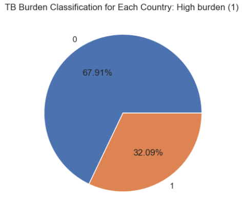
The data we were given generally contained information on the number and prevalence of TB cases across countries in different years. Specifically, it tracks metrics such as the estimated total population, TB prevalence and incidence rates (per 100,000 people), and the proportion of TB cases co-infected with HIV. This structured layout allows for both temporal trends and geographic disparities in TB burden to be thoroughly examined. Given this, we set on 2 different problems we are trying to solve : classifying whether a country, given the input parameters, is considered as one with high TB-burden in a given year and predicting the number of TB-cases for years beyond those given in the dataset.

Preprocessing the Dataset

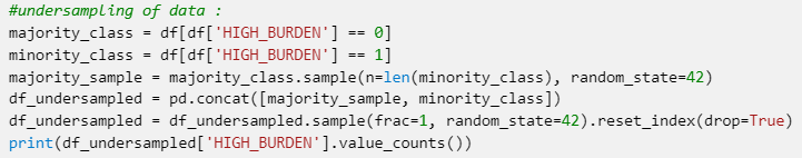
During preprocessing, we ensured absence of duplicates and null values in the dataset. When replacing the null values in the dataset, we decided to use mean as the number of outliers for each parameter is insignificant such that those outliers do not affect the calculation of the mean values. We also one hot encoded those features with categorical data such as Region through the code below.

We analysed the proportion of each class in the dataset and obtained the graph below.

Given the larger proportion of the countries classified as those with low TB Burden (labelled as 0) as compared to those with high TB Burden (labelled as 1), we decided to do an undersampling of the dataset as the initial imbalance in the dataset may affect the performance and accuracy of the model.

We also did feature correlation analysis and found that estimated prevalence of TB cases and estimated incidence of TB cases were the top 2 most correlated feature with high or low burden classification.

Decision Tree

Our initial model for this classification task was a Decision Tree, a widely used algorithm in machine learning that makes predictions by recursively splitting the data into branches based on feature values. Its intuitive, visual structure helps to reveal how different features contribute to decision-making.

In the first attempt, the model achieved an impressive F1-score of 98.58, indicating a high level of predictive performance. However, upon conducting a feature importance analysis, we observed that one feature (estimated incidence per 100,000 population) dominated the model. It had a disproportionately strong influence on the predictions, suggesting that the model’s high performance might be overly reliant on this single feature.

To address potential overfitting and to better assess the predictive value of the remaining features, we developed a second version of the model without this dominant feature. This revised model still performed well, achieving an F1-score of 95.13, which demonstrates strong predictive capability even without the most influential input.

This result suggests that while the dominant feature significantly boosts performance, the model retains meaningful predictive power from other features. It also indicates that our model is not entirely dependent on a single variable, supporting its robustness and potential generalizability to broader datasets or real-world applications.

Random Forest

Our second model is a Random Forest, which is a machine learning model that builds upon the decision tree approach. Unlike a single decision tree, which can be prone to overfitting, a Random Forest is an ensemble method that constructs multiple decision trees during training and aggregates their predictions to produce a final output. Here we also implemented the random forest using the scikit-learn (sklearn) library.

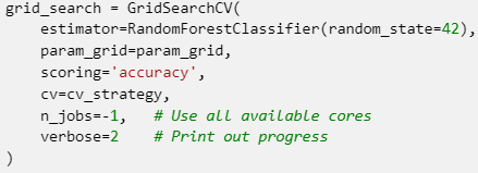
We trained the model using different combinations of hyperparameters and tested it using cross-validation with GridSearchCV, a method that systematically searches through a specified parameter grid to identify the optimal combination for model performance.

These parameters reveal some key insights about how the model was optimized:

1. By setting bootstrap=False, the model uses the entire training dataset (without sampling) to train each tree, which can improve stability when the dataset is not too large.

2. The choice of max_depth=None allows each decision tree to grow without a depth limit, enabling the model to capture more complex patterns in the data.

3. min_samples_leaf=1 permits leaf nodes to contain as few as one sample, which enhances sensitivity to fine-grained patterns.

4. At the same time, min_samples_split=5 adds a degree of regularization by preventing splits in nodes with fewer than five samples, reducing the risk of overfitting.

5. Lastly, n_estimators=50 specifies a relatively small ensemble of trees, which strikes a balance between computational efficiency and predictive performance.

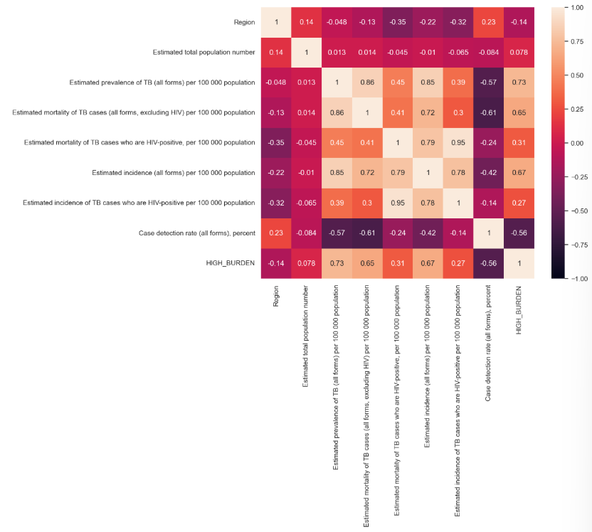
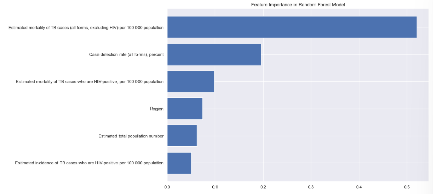
This model gave us an F1-score of 96.76% which is slightly higher than our decision tree model. The feature importance analysis further reveals that the model’s decisions are primarily driven by two key variables: “Estimated mortality of TB cases (excluding HIV) per 100,000 population” and “Case detection rate (all forms), percent”. These two features contributed the most to the model’s predictive power, with the former accounting for more than half of the total importance. This highlights their strong predictive relevance in determining TB burden levels.

XGBoost

Our third model is Extreme Gradient Boosting, or XGBoost, which is a powerful and scalable machine learning algorithm known for its performance and efficiency, especially on structured/tabular data. XGBoost is an implementation of gradient boosting that builds an ensemble of decision trees sequentially, where each new tree attempts to correct the errors made by the previous ones.

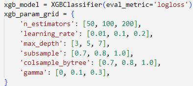
To optimize our XGBoost model, we conducted an extensive hyperparameter search using GridSearchCV with 5-fold cross-validation, evaluating performance based on accuracy. A total of 243 parameter combinations were tested across various values for learning rate, tree depth, subsample ratios, and regularization settings.

The best parameters identified were:

1. By setting n_estimators=200, the model builds a larger ensemble of trees, allowing it to learn more complex patterns and improve predictive accuracy.

2. The choice of learning_rate=0.2 provides a balanced learning pace—fast enough to converge efficiently, yet moderate enough to avoid overshooting during optimization.

3. max_depth=3 restricts the maximum depth of each tree, reducing the likelihood of overfitting while still capturing the essential structure of the data.

4. Setting subsample=0.8 means that each tree is trained on 80% of the training data, which introduces useful randomness and improves the model’s ability to generalize.

5. Similarly, colsample_bytree=0.8 limits the number of features considered for each tree to 80%, promoting diversity among the trees and further reducing overfitting.

6. Finally, gamma=0.3 applies a regularization constraint that penalizes unnecessary splits, encouraging simpler trees and helping to avoid fitting noise in the data.

These parameters collectively strike a balance between complexity and generalization. The tuned configuration led to a model that performed consistently well across folds.

The model gave us an F1-score of 98.2%, which is even higher than that of the previous Random Forest model. This indicates that XGBoost not only maintained a strong balance between precision and recall but also improved overall predictive performance. The boost in F1-score suggests that the model was better at correctly identifying both high and low TB burden cases, with fewer false positives and false negatives.

Based on our models, (write the conclusion)

Time Series Prediction

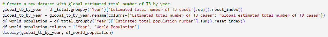
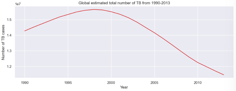
Another problem we tried to solve is predicting the Tuberculosis cases in the future. Here, we used ARIMA (Auto Regressive Integrated Moving Average) model. Since we are given the features estimated prevalence of TB cases per 100000 population for each country, we created the variable for storing the global estimated total number of TB cases for each year through the code below.

Given the data, we plotted the time series graph of global estimated total number of TB cases from 1990 to 2013 as shown in the graph below.

To evaluate the performance of our time series forecasting model for predicting TB cases, we adopted a temporal train-test split approach that mirrors real-world prediction scenarios. Specifically, we used data from 2000 to 2012 as the training set, allowing the model to learn historical trends and patterns. The year 2013 was set aside as the test set.

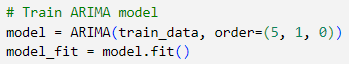
To forecast the global number of TB cases, we used an ARIMA(5, 1, 0) model. Here, the model leverages the past 5 time steps (p=5) to predict the current value, capturing short-term dependencies through its autoregressive component. The first-order differencing (d=1) step ensures the series is stationary by removing trends, which is crucial for ARIMA models to perform accurately. We set the moving average term (q=0) to zero, meaning we rely entirely on the autoregressive part without smoothing past forecast errors.

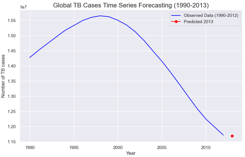
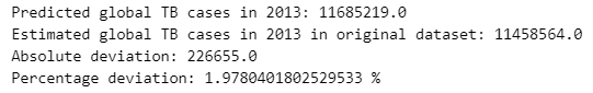
Once trained, ARIMA model relies on the autoregressive (AR) coefficients it learned during training to make this prediction. The forecasted value in this case is the sum of the 5 past weighted lagged values since we set p=5 earlier. Then the model reverses the differencing step to return the prediction to its original scale. This gives us an estimate for the actual number of TB cases in 2013. A graph of the predicted TB cases in 2013 is as shown.

After calculating the deviation from the actual value, we obtained a percentage deviation of 1.98%.

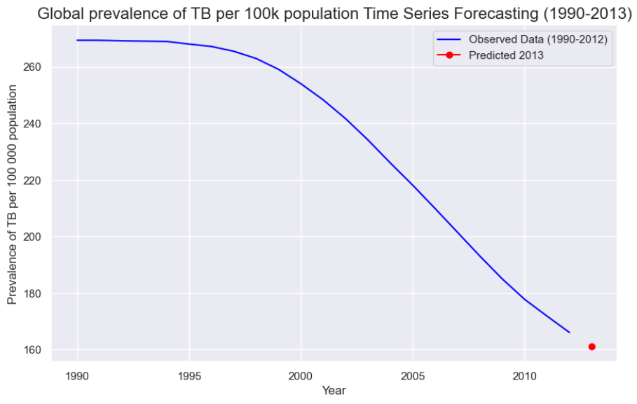
We then decided to do a second approach on the arima model but this time with the estimated global prevalence of TB cases per 100,000 population for each year.

After conducting the prediction, we obtained the graph as shown below.

For this model, we obtained a percentage deviation of 31% which is lower than the previous model.

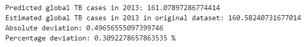
The difference in accuracy between the two ARIMA models can be explained by the underlying characteristics of the target variables they are trained on. The model predicting TB prevalence per 100,000 population works with a normalized and relatively stable time series, which tends to be smoother and more stationary which are conditions that suit ARIMA models well. In contrast, the model forecasting the total number of TB cases deals with a raw count that is influenced by population growth, data reporting inconsistencies, and larger year-to-year fluctuations, making the series more volatile and harder to model effectively.

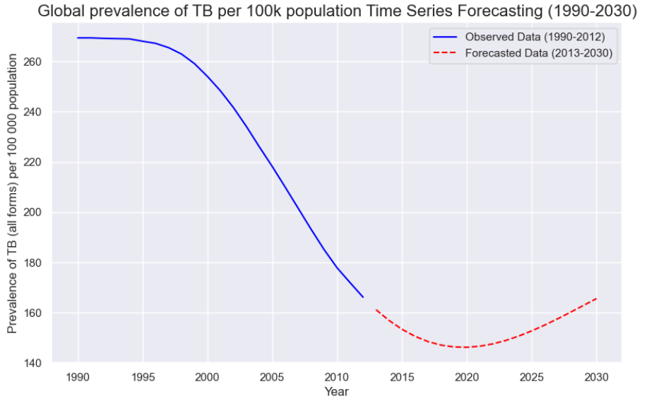
Based on the second model, we made a prediction on the estimated global prevalence of TB cases per 100,000 population until 2030 and obtained the graph as shown below.

Acknowledgment:

This project was done in collaboration with three of my teammates who contributed significantly to various parts of the work, including data preprocessing and time series modelling.